Quadrupedal jump example of robotoc::OCPSolver in Python

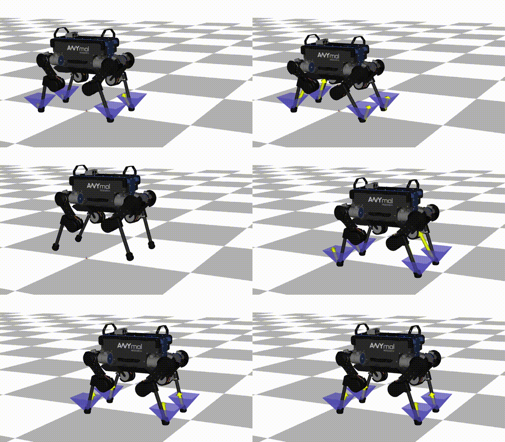
This page explains the example code in examples/anymal/python/jump.py.

Required imports are as follows.

import robotoc
import numpy as np
import math

First, we define the robot model. We speficy the URDF path, base joint type, and contact frames (in this case, the contact frames are the frames of all feet).

model_info = robotoc.RobotModelInfo()
model_info.urdf_path = '../anymal_b_simple_description/urdf/anymal.urdf'
model_info.base_joint_type = robotoc.BaseJointType.FloatingBase
baumgarte_time_step = 0.05
model_info.point_contacts = [robotoc.ContactModelInfo('LF_FOOT', baumgarte_time_step),
                             robotoc.ContactModelInfo('LH_FOOT', baumgarte_time_step),
                             robotoc.ContactModelInfo('RF_FOOT', baumgarte_time_step),
                             robotoc.ContactModelInfo('RH_FOOT', baumgarte_time_step)]
robot = robotoc.Robot(model_info)

Note

baumgarte_time_step is the stabilization parameter for acceleration-level rigid contact constraints. The best choice of baumgarte_time_step may be the time step of the optimal control problem. However, it is often too small to make the optimization problem high nonlinear. A moderate value such as several times of the time step of optimal control problem may be sufficient

Then set the parameters for the optimal control problem of the jump motion such as the jump length

dt = 0.01
jump_length = np.array([0.5, 0, 0])
jump_height = 0.1
flying_up_time = 0.15
flying_down_time = flying_up_time
flying_time = flying_up_time + flying_down_time
ground_time = 0.30
t0 = 0

Next, we construct the cost function (TODO: write details about the cost function components).

cost = robotoc.CostFunction()
q_standing = np.array([0, 0, 0.4792, 0, 0, 0, 1, 
                       -0.1,  0.7, -1.0, 
                       -0.1, -0.7,  1.0, 
                        0.1,  0.7, -1.0, 
                        0.1, -0.7,  1.0])
q_weight = np.array([0, 0, 0, 250000, 250000, 250000, 
                     0.0001, 0.0001, 0.0001, 
                     0.0001, 0.0001, 0.0001,
                     0.0001, 0.0001, 0.0001,
                     0.0001, 0.0001, 0.0001])
v_weight = np.array([100, 100, 100, 100, 100, 100, 
                     1, 1, 1, 
                     1, 1, 1,
                     1, 1, 1,
                     1, 1, 1])
u_weight = np.full(robot.dimu(), 1.0e-01)
q_weight_impact = np.array([1.0, 1.0, 1.0, 1.0, 1.0, 1.0, 
                      100, 100, 100, 
                      100, 100, 100,
                      100, 100, 100,
                      100, 100, 100])
v_weight_impact = np.full(robot.dimv(), 100)
config_cost = robotoc.ConfigurationSpaceCost(robot)
config_cost.set_q_ref(q_standing)
config_cost.set_q_weight(q_weight)
config_cost.set_q_weight_terminal(q_weight)
config_cost.set_q_weight_impact(q_weight_impact)
config_cost.set_v_weight(v_weight)
config_cost.set_v_weight_terminal(v_weight)
config_cost.set_v_weight_impact(v_weight_impact)
config_cost.set_u_weight(u_weight)
cost.add("config_cost", config_cost)
 
robot.forward_kinematics(q_standing)
x3d0_LF = robot.frame_position('LF_FOOT')
x3d0_LH = robot.frame_position('LH_FOOT')
x3d0_RF = robot.frame_position('RF_FOOT')
x3d0_RH = robot.frame_position('RH_FOOT')
 
com_ref0_flying_up = robot.com()
vcom_ref_flying_up = 0.5*jump_length/flying_up_time + np.array([0, 0, (jump_height/flying_up_time)])
com_ref_flying_up = robotoc.PeriodicCoMRef(com_ref0_flying_up, vcom_ref_flying_up, 
                                           t0+ground_time, flying_up_time, 
                                           flying_down_time+2*ground_time, False)
com_cost_flying_up = robotoc.CoMCost(robot, com_ref_flying_up)
com_cost_flying_up.set_weight(np.full(3, 1.0e06))
cost.add("com_cost_flying_up", com_cost_flying_up)
 
com_ref0_landed = robot.com()
com_ref0_landed += jump_length
vcom_ref_landed = np.zeros(3)
com_ref_landed = robotoc.PeriodicCoMRef(com_ref0_landed, vcom_ref_landed, 
                                        t0+ground_time+flying_time, ground_time, 
                                        ground_time+flying_time, False)
com_cost_landed = robotoc.CoMCost(robot, com_ref_landed)
com_cost_landed.set_weight(np.full(3, 1.0e06))
cost.add("com_cost_landed", com_cost_landed)

Next, we construct the constraints.

constraints           = robotoc.Constraints(barrier=1.0e-03, fraction_to_boundary_rule=0.995)
joint_position_lower  = robotoc.JointPositionLowerLimit(robot)
joint_position_upper  = robotoc.JointPositionUpperLimit(robot)
joint_velocity_lower  = robotoc.JointVelocityLowerLimit(robot)
joint_velocity_upper  = robotoc.JointVelocityUpperLimit(robot)
joint_torques_lower   = robotoc.JointTorquesLowerLimit(robot)
joint_torques_upper   = robotoc.JointTorquesUpperLimit(robot)
friction_cone         = robotoc.FrictionCone(robot)
constraints.add("joint_position_lower", joint_position_lower)
constraints.add("joint_position_upper", joint_position_upper)
constraints.add("joint_velocity_lower", joint_velocity_lower)
constraints.add("joint_velocity_upper", joint_velocity_upper)
constraints.add("joint_torques_lower", joint_torques_lower)
constraints.add("joint_torques_upper", joint_torques_upper)
constraints.add("friction_cone", friction_cone)

Next, we construct the contact sequence robotoc::ContactSequence as

contact_sequence = robotoc.ContactSequence(robot)

We set the contact positions and friction coefficients through the contact sequence. We then define the friction coefficients.

mu = 0.7
friction_coefficients = {'LF_FOOT': mu, 'LH_FOOT': mu, 'RF_FOOT': mu, 'RH_FOOT': mu} 

We set the initial contact status of the robot. In the beginning, the robot is standing, so all the contacts are active.

contact_positions = {'LF_FOOT': x3d0_LF, 'LH_FOOT': x3d0_LH, 'RF_FOOT': x3d0_RF, 'RH_FOOT': x3d0_RH} 
contact_status_standing = robot.create_contact_status()
contact_status_standing.activate_contacts(['LF_FOOT', 'LH_FOOT', 'RF_FOOT', 'RH_FOOT'])
contact_status_standing.set_contact_placements(contact_positions)
contact_status_standing.set_friction_coefficients(friction_coefficients)
contact_sequence.init(contact_status_standing)

Next, we set the contact status when the robot is flying. Then the all the contacts are inactive.

contact_status_flying = robot.create_contact_status()
contact_sequence.push_back(contact_status_flying, t0+ground_time)

Then a lift event is automatically appended into the contact sequence. Finally, we set the contact status after touch-down as

contact_positions['LF_FOOT'] += jump_length
contact_positions['LH_FOOT'] += jump_length
contact_positions['RF_FOOT'] += jump_length
contact_positions['RH_FOOT'] += jump_length
contact_status_standing.set_contact_placements(contact_positions)
contact_sequence.push_back(contact_status_standing, t0+ground_time+flying_time)

Then an impact event is automatically appended into the contact sequence.

Note

We can check the contact sequence via

print(contact_sequence)

Finally, we can construct the optimal control solver!

T = t0 + flying_time + 2*ground_time
N = math.floor(T/dt) 
ocp = robotoc.OCP(robot=robot, cost=cost, constraints=constraints, 
                  contact_sequence=contact_sequence, T=T, N=N)
solver_options = robotoc.SolverOptions()
solver_options.nthreads = 4
ocp_solver = robotoc.OCPSolver(ocp=ocp, solver_options=solver_options)

Let's run the solver!

t = 0.
q = q_standing # initial state.
v = np.zeros(robot.dimv()) # initial state.
 
ocp_solver.discretize(t) # discretizes the optimal control problem.
ocp_solver.set_solution("q", q) # set the initial guess of the solution.
ocp_solver.set_solution("v", v) # set the initial guess of the solution.
f_init = np.array([0.0, 0.0, 0.25*robot.total_weight()])
ocp_solver.set_solution("f", f_init) # set the initial guess of the solution.
 
ocp_solver.init_constraints() # initialize the slack and dual variables of the primal-dual interior point method.
print("Initial KKT error: ", ocp_solver.KKT_error(t, q, v))
ocp_solver.solve(t, q, v)
print("KKT error after convergence: ", ocp_solver.KKT_error(t, q, v)) 
print(ocp_solver.get_solver_statistics()) # print solver statistics

We can visualize the solution trajectory as

viewer = robotoc.utils.TrajectoryViewer(model_info=model_info, viewer_type='gepetto')
viewer.set_contact_info(mu=mu)
viewer.display(ocp_solver.get_time_discretization(), 
               ocp_solver.get_solution('q'), 
               ocp_solver.get_solution('f', 'WORLD'))

Note

We can check the discretization of the optimal control problem sololy via

time_discretization = robotoc.TimeDiscretization(T, N)
time_discretization.discretize(contact_sequence, t)
print(time_discretization)