Switching time optimization (STO) example of robotoc::OCPSolver in Python

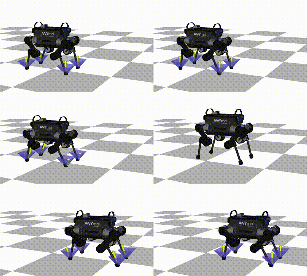
This page explains the example code in examples/anymal/python/jump_sto.py.

Required imports are as follows.

import robotoc
import numpy as np
import math

First, we define the robot model. We speficy the URDF path, base joint type, and contact frames (in this case, the contact frames are the frames of all feet).

model_info = robotoc.RobotModelInfo()
model_info.urdf_path = '../anymal_b_simple_description/urdf/anymal.urdf'
model_info.base_joint_type = robotoc.BaseJointType.FloatingBase
baumgarte_time_step = 0.05
model_info.point_contacts = [robotoc.ContactModelInfo('LF_FOOT', baumgarte_time_step),
                             robotoc.ContactModelInfo('LH_FOOT', baumgarte_time_step),
                             robotoc.ContactModelInfo('RF_FOOT', baumgarte_time_step),
                             robotoc.ContactModelInfo('RH_FOOT', baumgarte_time_step)]
robot = robotoc.Robot(model_info)

Note

baumgarte_time_step is the stabilization parameter for acceleration-level rigid contact constraints. The best choice of baumgarte_time_step may be the time step of the optimal control problem. However, it is often too small to make the optimization problem high nonlinear. A moderate value such as several times of the time step of optimal control problem may be sufficient

Then set the parameters for the optimal control problem of the jump motion such as the jump length

dt = 0.02
jump_length = np.array([0.8, 0, 0])
flying_up_time = 0.15
flying_down_time = flying_up_time
flying_time = flying_up_time + flying_down_time
ground_time = 0.7
t0 = 0.

Next, we construct the cost function. The below is the simple quadratic cost for the optimization variables.

cost = robotoc.CostFunction()
q_standing = np.array([0., 0., 0.4792, 0., 0., 0., 1.0, 
                       -0.1,  0.7, -1.0, 
                       -0.1, -0.7,  1.0, 
                        0.1,  0.7, -1.0, 
                        0.1, -0.7,  1.0])
q_ref = q_standing.copy()
q_ref[0] += jump_length
q_weight = np.array([1.0, 0., 0., 1.0, 1.0, 1.0, 
                     0.001, 0.001, 0.001, 
                     0.001, 0.001, 0.001,
                     0.001, 0.001, 0.001,
                     0.001, 0.001, 0.001])
v_weight = np.full(robot.dimv(), 1.0)
a_weight = np.full(robot.dimv(), 1.0e-06)
q_weight_impact = np.array([0., 0., 0., 100., 100., 100., 
                      0.1, 0.1, 0.1, 
                      0.1, 0.1, 0.1,
                      0.1, 0.1, 0.1,
                      0.1, 0.1, 0.1])
v_weight_impact = np.full(robot.dimv(), 1.0)
dv_weight_impact = np.full(robot.dimv(), 1.0e-06)
config_cost = robotoc.ConfigurationSpaceCost(robot)
config_cost.set_q_ref(q_ref)
config_cost.set_q_weight(q_weight)
config_cost.set_q_weight_terminal(q_weight)
config_cost.set_q_weight_impact(q_weight_impact)
config_cost.set_v_weight(v_weight)
config_cost.set_v_weight_terminal(v_weight)
config_cost.set_v_weight_impact(v_weight_impact)
config_cost.set_dv_weight_impact(dv_weight_impact)
config_cost.set_a_weight(a_weight)
cost.add("config_cost", config_cost)

Next, we construct the constraints.

constraints           = robotoc.Constraints(barrier_param=1.0e-03, fraction_to_boundary_rule=0.995)
joint_position_lower  = robotoc.JointPositionLowerLimit(robot)
joint_position_upper  = robotoc.JointPositionUpperLimit(robot)
joint_velocity_lower  = robotoc.JointVelocityLowerLimit(robot)
joint_velocity_upper  = robotoc.JointVelocityUpperLimit(robot)
joint_torques_lower   = robotoc.JointTorquesLowerLimit(robot)
joint_torques_upper   = robotoc.JointTorquesUpperLimit(robot)
friction_cone         = robotoc.FrictionCone(robot)
constraints.add("joint_position_lower", joint_position_lower)
constraints.add("joint_position_upper", joint_position_upper)
constraints.add("joint_velocity_lower", joint_velocity_lower)
constraints.add("joint_velocity_upper", joint_velocity_upper)
constraints.add("joint_torques_lower", joint_torques_lower)
constraints.add("joint_torques_upper", joint_torques_upper)
constraints.add("friction_cone", friction_cone)

Next, we construct the contact sequence robotoc::ContactSequence as

contact_sequence = robotoc.ContactSequence(robot)

Then we can set an impact event and a lift event to the contact sequence.

We set the contact positions and friction coefficients through the contact sequence. We then define the friction coefficients.

mu = 0.7
friction_coefficients = {'LF_FOOT': mu, 'LH_FOOT': mu, 'RF_FOOT': mu, 'RH_FOOT': mu} 

We set the initial contact status of the robot. In the beginning, the robot is standing, so all the contacts are active.

robot.forward_kinematics(q_standing)
x3d0_LF = robot.frame_position('LF_FOOT')
x3d0_LH = robot.frame_position('LH_FOOT')
x3d0_RF = robot.frame_position('RF_FOOT')
x3d0_RH = robot.frame_position('RH_FOOT')
contact_positions = {'LF_FOOT': x3d0_LF, 'LH_FOOT': x3d0_LH, 'RF_FOOT': x3d0_RF, 'RH_FOOT': x3d0_RH} 
 
contact_status_standing = robot.create_contact_status()
contact_status_standing.activate_contacts(['LF_FOOT', 'LH_FOOT', 'RF_FOOT', 'RH_FOOT'])
contact_status_standing.set_contact_placements(contact_positions)
contact_status_standing.set_friction_coefficients(friction_coefficients)
contact_sequence.init(contact_status_standing)

Next, we set the contact status when the robot is flying. Then the all the contacts are inactive.

contact_status_flying = robot.create_contact_status()
contact_sequence.push_back(contact_status_flying, t0+ground_time-0.3, sto=True)

Then a lift event is automatically appended into the contact sequence. By setting sto=True, the switching time of this event is regarded as an optimization variable. Finally, we set the contact status after touch-down as

contact_positions['LF_FOOT'] += jump_length
contact_positions['LH_FOOT'] += jump_length
contact_positions['RF_FOOT'] += jump_length
contact_positions['RH_FOOT'] += jump_length
contact_status_standing.set_contact_placements(contact_positions)
contact_sequence.push_back(contact_status_standing, t0+ground_time+flying_time-0.1, sto=True)

Then an impact event is automatically appended into the contact sequence.

Note

We can check the contact sequence via

print(contact_sequence)

We further construct cost function for the switching time optimization (STO) problem

sto_cost = robotoc.STOCostFunction()

and the minimum dwell-time constraints for the STO problem

sto_constraints = robotoc.STOConstraints(minimum_dwell_times=[0.15, 0.15, 0.65],
                                         barrier_param=1.0e-03, 
                                         fraction_to_boundary_rule=0.995)

Finally, we can construct the optimal control solver!

T = t0 + flying_time + 2*ground_time
N = math.floor(T/dt) 
ocp = robotoc.OCP(robot=robot, contact_sequence=contact_sequence, 
                  cost=cost, constraints=constraints, 
                  sto_cost=sto_cost, sto_constraints=sto_constraints, T=T, N=N)
solver_options = robotoc.SolverOptions()
solver_options.kkt_tol_mesh = 0.1
solver_options.max_dt_mesh = T/N 
solver_options.max_iter = 200
solver_options.nthreads=4
ocp_solver = robotoc.OCPSolver(ocp=ocp, solver_options=solver_options)

Note

Without robotoc::STOCostFunction and robotoc::STOConstraints, the solver does not optimize the switching times. Therefore, even if there are empty (e.g., the STO cost of this example is also empty), please pass them to the constructor of OCP.

In this example, we want to optimize the switching times as well as the whole-body trajectory of the robot. Then we need to carry on mesh refinement because the switching times change over the iterations. We set SolverOptions::max_dt_mesh that the maximum value of the time-steps. We also set SolverOptions::kkt_tol_mesh and we apply the mesh refinement when the KKT error is less than SolverOptions::kkt_tol_mesh and the maximum time step is larger than SolverOptions::max_dt_mesh.

Let's run the solver!

t = 0.
q = q_standing # initial state.
v = np.zeros(robot.dimv()) # initial state.
 
ocp_solver.discretize(t) # discretizes the optimal control problem.
ocp_solver.setSolution("q", q); # set the initial guess of the solution.
ocp_solver.setSolution("v", v); # set the initial guess of the solution.
Eigen::Vector3d f_init;
f_init << 0, 0, 0.25*robot.totalWeight();
ocp_solver.setSolution("f", f_init); # set the initial guess of the solution.
 
ocp_solver.init_constraints() # initialize the slack and dual variables of the primal-dual interior point method.
print("Initial KKT error: ", ocp_solver.KKT_error(t, q, v))
ocp_solver.solve(t, q, v)
print("KKT error after convergence: ", ocp_solver.KKT_error(t, q, v)) 
print(ocp_solver.get_solver_statistics()) # print solver statistics

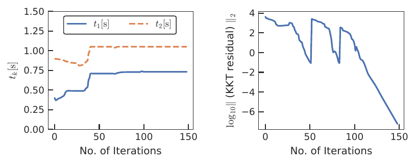
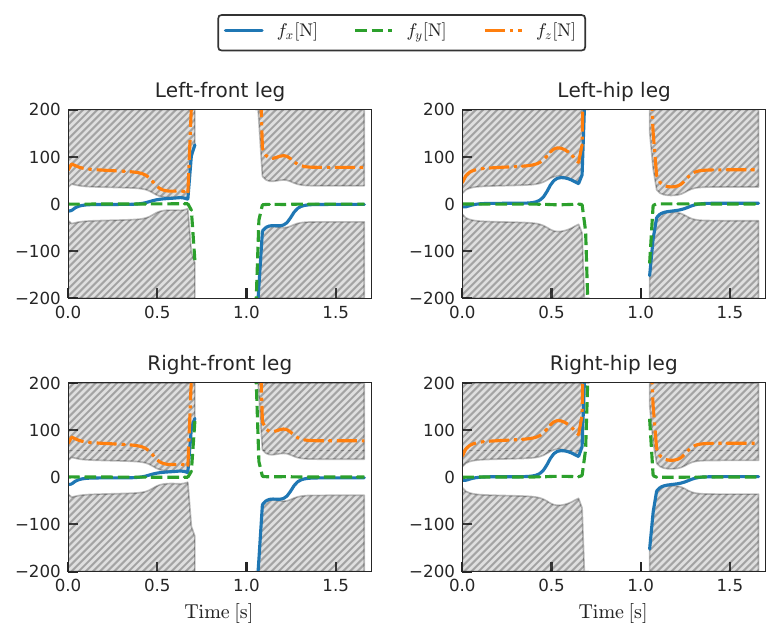
We can plot the convergence and the optimal contact forces as

kkt_data = ocp_solver.get_solver_statistics().kkt_error + [ocp_solver.KKT_error()] # append KKT after convergence
ts_data = ocp_solver.get_solver_statistics().ts + [contact_sequence.event_times()] # append ts after convergence
 
plot_ts = robotoc.utils.PlotConvergence()
plot_ts.ylim = [0., 1.5]
plot_ts.plot(kkt_data=kkt_data, ts_data=ts_data, fig_name='jump_sto', 
             save_dir='jump_sto_log')
 
plot_f = robotoc.utils.PlotContactForce(mu=mu)
plot_f.plot(f_data=ocp_solver.get_solution('f', 'WORLD'), 
            t=ocp_solver.get_time_discretization().time_points(), 
            fig_name='jump_sto_f', save_dir='jump_sto_log')

Then we obtain the convergence results ((left) switching times and (right) KKT error at each iteration)

and the solution trajectory of the contact forces

where the grey hatches indicates the infeasible regions of fx and fy due to the friction cone constraints. We can see that the solution strictly satisfies the friction cone constraints.

We can also visualize the solution trajectory as

viewer = robotoc.utils.TrajectoryViewer(path_to_urdf=path_to_urdf, 
                                        base_joint_type=robotoc.BaseJointType.FloatingBase,
                                        viewer_type='gepetto')
viewer.set_contact_info(robot.contact_frames(), mu)
viewer.display(ocp_solver.get_time_discretization().time_steps(), 
               ocp_solver.get_solution('q'), 
               ocp_solver.get_solution('f', 'WORLD'))

Note

We can check the discretization of the optimal control problem sololy via

time_discretization = robotoc.TimeDiscretization(T, N)
time_discretization.discretize(contact_sequence, t)
print(time_discretization)